The 4 Basic Types of Time Complexity

Time complexity is a measure of the number of operations an algorithm must make in relation to the number of inputs we give it. We call the number of inputs n. We use the term marginal cost to describe the increase in runtime caused by increasing n by 1.

For example, an each function has a linear time complexity, since it needs to go through each value in the collection once. The time it takes to run that algorithm increases by 1 as the size of that collection increases, meaning that it has a marginal cost of 1. In Big O notation we would say that an each function is O(n).

[1, 2, 3].each(function (val) {
  console.log(val);
});

There are four basic types of time complexity: constant time (O(1)), linear time (O(n)), logarithmic time (O(log n)) and quadratic time (O(n²)). If you were to graph them, they would look something like this:

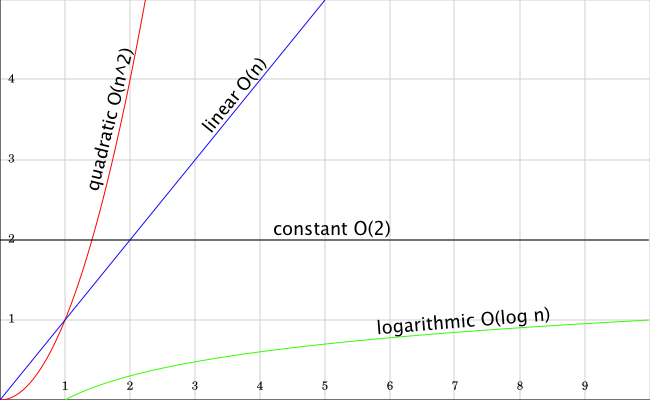
In the graph, the x axis represents the size of n (or algorithm input) and y represents (in relative terms) the amount of time it would take to execute that algorithm.

Let’s run through some examples for each type of time complexity:

Constant Time: O(1)

These are algorithms that have a marginal cost of 0, since they always take the same time, independently of the size of n. An example of this is accessing a property in a JavaScript object. Accessing a['jorge'] will always take the same time, independently of the size of our a object.

a['jorge']

Linear Time: O(n)

Linear time algorithms have a marginal cost of 1, meaning that their increase in execution time is directly proportional to n. A for loop is a perfect example of this. The time it takes to execute a for loop will increase linearly as the size of n increases.

// You know how a for loop works!
for (var i = 0; i < n; i +=1 {
  console.log(i);
}

Logarithmic Time: O(log n)

Logarithmic algorithms have a decreasing marginal cost.

It’s execution time increases by log(n) (less than 1) as the size of n increases. An example of this is a looking up a value in a binary tree. The lookup time on a binary tree will grow at a lower rate as new nodes are added to the binary tree.

If we wanted to find 11, for example, we would only need to go through 3 values (10, 15, 11).

                       *10*
                     /      \
                   5        *15*
                 /   \      /   \
               1      7   *11*   17

Quadratic Time: O(n²)

Algorithms with quadratic time have a marginal cost of n². The algorithm’s execution time increases exponentially as the size of n increases. An example of this is a bubble sort. In this sorting algorithm, every time a node is added the algorithm must go through each value in n one more time, making the addition of that node very expensive.

Here you can see how bubble sort loops through every value and then goes through every value again.

var bubbleSort = function (collection, iterator) {
    var n = collection.length;
    var swapped = true;
    /*
     * Loop through each value O(n)
     */
    while (swapped !== false) {
      swapped = false;
      /*
       * Loop through each value O(n)
       */
      for (var i = 1; i < n; i += 1) {
      // if this pair is out of order
      if (collection[i - 1] > collection[i]
      || !collection[i - 1] && collection[i]
      ){
        collection = swap(collection, (i - 1), i);
        swapped = true;
      }
    }
  }
  return collection;
};

There it is! Hope this was a helpful introduction to time complexity. Thanks to my good friend Brian Scoles for revising this blog post and letting me steal some of his language.D